Tool showcase
To showcase the toolbox applications and facilitate the understanding of the methods, we provide examples for the analysis of two datasets presented in our preprint. Those datasets can be download with the following commands from within a nanodisco container: get_data_bacteria and get_data_microbiome.
Prepare the container for examples
singularity build --sandbox nd_example nanodisco.sif # Create a writable container (directory) named nd_example
singularity run --no-home -w nd_example              # Start an interactive shell to use nanodisco, type `exit` to leave
Note
The image retrieved from Singularity Hub with singularity pull (e.g. nanodisco.sif) is already built and can be reused at will. The command singularity build creates a container from the image as a writable directory called a sandbox (nd_example). The command singularity run starts an interactive shell within the nd_example container. You can directly reuse the same sandbox directory or you can create multiple sandbox directories to compartmentalize analysis of different datasets (e.g. my_analysis and my_analysis2). Containers built with those instructions are writable meaning that results from nanodisco analysis can be retrieved when the container is not running. Outputs for the following commands can be found at ./path/to/nd_example/home/nanodisco/analysis.
Methylation typing and fine mapping
Goal: Identify the specific type (6mA, 5mC or 4mC, namely typing) of a methylation motif, and identify which specific position within the motif is methylated (namely fine mapping). The detailed method is described in the preprint.
Inputs:
- Current differences file (pre-computed in the following example, can be generated with
nanodisco difference) - Reference genome file (.fasta)
- Methylation motifs for which one wants to perform typing and fine mapping
Outputs: For each queried methylation motif, nanodisco identifies the methylation type and the methylated position summarized in a heatmap (analysis/Ecoli_motifs/Motifs_classification_Ecoli_nn_model.pdf). See Figure 4d in the preprint as an example. In addition, the predicted methylation type and methylated position for each motif is compiled in a text file (analysis/Ecoli_motifs/Motifs_classification_Ecoli_nn_model.tsv).
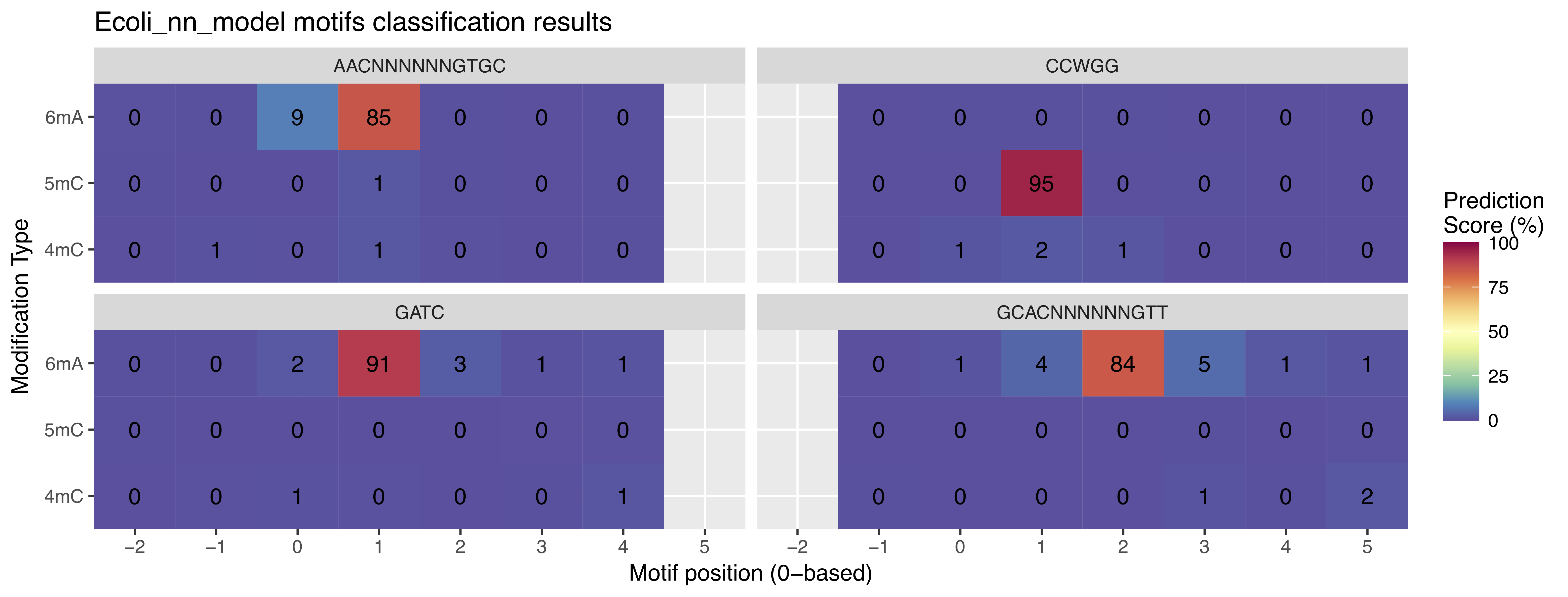
Interpretation of the above figure
- AACNNNNNNGTGC: highest value (85) is on the 6mA row with offset +1 (relative to the first base), meaning that the second base (A) is 6mA
- CCWGG: highest value (95) is on the 5mC row with offset +1 (relative to the first base), meaning that the second base (C) is 5mC
- GATC: highest value (91) is on the 6mA row with offset +1 (relative to the first base), meaning that the second base (A) is 6mA
- GCACNNNNNNGTT: highest value (84) is on the 6mA row with offset +2 (relative to the first base), meaning that the third base (A) is 6mA
Example commands:
get_data_bacteria # Retrieve E. coli current differences and reference genome
nanodisco characterize -p 4 -b Ecoli -d dataset/EC_difference.RDS -o analysis/Ecoli_motifs -m GATC,CCWGG,GCACNNNNNNGTT,AACNNNNNNGTGC -t nn -r reference/Ecoli_K12_MG1655_ATCC47076.fasta
See details and advanced parameters in characterize section. In this example, the current differences file (EC_difference.RDS) was generated on a whole E. coli nanopore sequencing dataset, from the preprint, using nanodisco difference. Runtime is ~1 min with 4 threads (~6.5 GB memory used).
Methylation binning of metagenomic contigs
Goal: Construct methylation profiles for metagenomic contigs, identify informative features, and perform methylation binning for high-resolution metagenomic analysis.
Inputs:
- Current differences file (pre-computed in the following example)
- Metagenomic de novo assembly (.fasta)
- Metagenomic contigs coverage files (pre-computed in the following example)
- De novo discovered methylation motifs (pre-computed in the following example)
- (Optional) Annotation for metagenome contigs (e.g. species of origin) and List of contigs from Mobile Genetic Elements (MGEs)
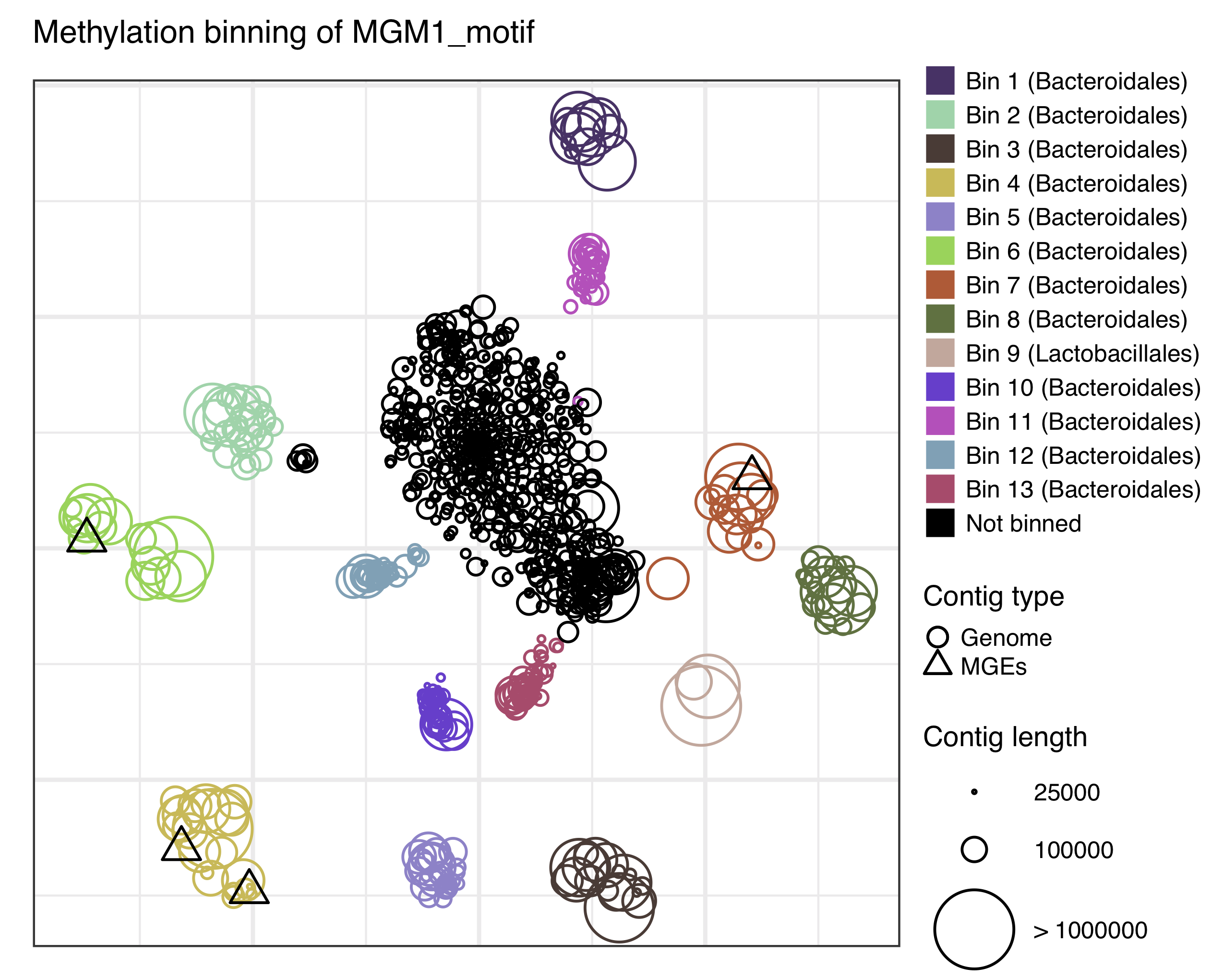
Outputs: t-SNE scatter plot that demonstrates the species level clustering of metagenomic contigs (analysis/binning/Contigs_methylation_tsne_MGM1_motif.pdf) as presented in Figure 5a in the preprint. Optionally, binned fasta files can be generated.
Example commands:
get_data_microbiome # Retrieve current differences, de novo metagenome assembly, etc
nanodisco profile -p 4 -r reference/metagenome.fasta -d dataset/metagenome_subset_difference.RDS -w dataset/metagenome_WGA.cov -n dataset/metagenome_NAT.cov -b MGM1_motif -o analysis/binning --motifs_file dataset/list_de_novo_discovered_motifs.txt
nanodisco binning -r reference/metagenome.fasta -s dataset/methylation_profile_MGM1_motif.RDS -b MGM1_motif -o analysis/binning
nanodisco plot_binning -r reference/metagenome.fasta -u analysis/binning/methylation_binning_MGM1_motif.RDS -b MGM1_motif -o analysis/binning -a reference/motif_binning_annotation.RDS --MGEs_file dataset/list_MGE_contigs.txt
See details and advanced parameters in profile, binning, and plot_binning sections. In this example, the current differences file (metagenome_subset_difference.RDS) was generated on a mouse gut microbiome nanopore sequencing dataset, MGM1 from the preprint, using nanodisco difference. This example corresponds to the procedure referred to as guided methylation binning where methylation motifs were already de novo discovered. Runtime is ~10 min with 4 threads and ~4 GB of memory used. We also described the procedure for automated methylation binning (including methylation features selection) from current differences file to binning results in the detailed tutorial.